Basic Knowledge of Robot

4.1 Introduction to this chapter

This chapter introduces the basic knowledge of the robot. Familiarity with the contents of this chapter will help to better understand and master the use of the control system and robot.

4.2 Frame

Any object (tool, work object, etc.) in space has six degrees of freedom (DOF): three translational degrees of freedom and three rotational degrees of freedom. The three translational degrees of freedom constitute the position; the three rotational degrees of freedom constitute the orientation; and these six degrees of freedom are collectively referred to as pose. The pose of an object can be described by the frame attached to it, generally using the Cartesian frame (hereinafter referred to as the "frame").

The robot is a mechanism with multiple degrees of freedom. Its typical operation mode is to use a tool attached to the flange to execute the movements relative to external work objects. This mode of operation can be described through the frame and its relative motion.

The frames currently used in the xCore system are shown below:

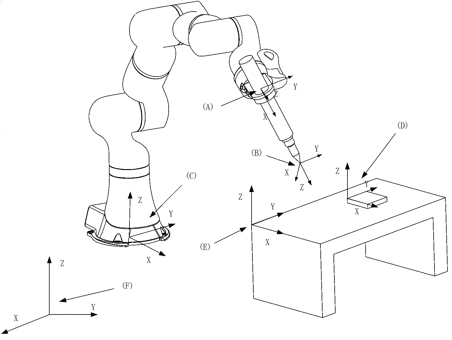
No.	Frame	Meaning
A	Flange frame	Defined in the center of the robot flange; The flange frame is defined relative to the base frame;
B	Tool frame	Defined at the end of the tool; When the tool is a handheld tool (ordinary tool), the tool frame is defined relative to the flange frame; and when the tool is an external tool, the tool frame is defined relative to the user frame;
C	Base frame	Defined in the center of the robot base; The base frame is defined relative to the world frame. Note: If the robot is not installed in the default way, such as upside-down or slanted installation, the base frame needs to be calibrated first;
D	Work object frame	Defined in the work object; When the work object is an external work object (ordinary work object), the work object frame is defined relative to the user frame; and when the work object is a handheld work object, the work object frame is defined relative to the flange frame;
E	User frame	The user frame is used as a reference when defining the work object frame, and it cannot be used separately; The user frame is defined relative to the world frame;
F	World frame	The world frame is generally used as the reference frame and has no specific position. When a single robot is installed normally, it coincides with the robot base frame by default; and when multiple robots or external devices are involved in collaboration, the unification of motion reference can be achieved by unifying their world frames into a same frame;

No.

Frame

Meaning

Flange frame

Defined in the center of the robot flange;

The flange frame is defined relative to the base frame;

Tool frame

Defined at the end of the tool;

When the tool is a handheld tool (ordinary tool), the tool frame is defined relative to the flange frame; and when the tool is an external tool, the tool frame is defined relative to the user frame;

Base frame

Defined in the center of the robot base;

The base frame is defined relative to the world frame.

Note: If the robot is not installed in the default way, such as upside-down or slanted installation, the base frame needs to be calibrated first;

Work object frame

Defined in the work object;

When the work object is an external work object (ordinary work object), the work object frame is defined relative to the user frame; and when the work object is a handheld work object, the work object frame is defined relative to the flange frame;

User frame

The user frame is used as a reference when defining the work object frame, and it cannot be used separately;

The user frame is defined relative to the world frame;

World frame

The world frame is generally used as the reference frame and has no specific position. When a single robot is installed normally, it coincides with the robot base frame by default; and when multiple robots or external devices are involved in collaboration, the unification of motion reference can be achieved by unifying their world frames into a same frame;

4.3 Singularity

There are a few special poses in the robot’s working space that the robot can arrive at using a myriad of different joint configurations. Such poses are called singularities. Singularities may cause problems to the control system when calculating joint angles based on Cartesian space pose.

There are no singularity problems when the robot performs joint motion.

When the robot executes a Cartesian space trajectory near a singular point, the speed of some joints may be very fast, potentially leading to an error report and subsequent cessation of the robot’s operation.

4.3.1 Typical singular positions of robots

Robots with different configurations have different singular positions. Typical singular positions of some robot configurations are described below.

4.3.1.1 Singular position of the six-axis industrial robot

Singularity	Configuration	Explanation
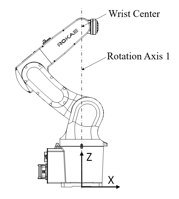
Shoulder singularity		When the robot’s wrist center is located on the Axis 1.
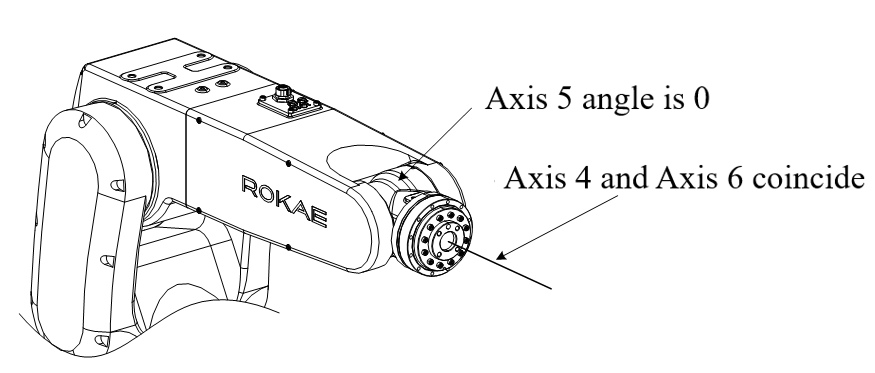
Wrist singularity		When the Axis 4 and Axis 6 coincide (Axis 5 angle is 0).
Elbow singularity		When the wrist center, Rotation Axis 2, and Rotation Axis 3 are in a straight line.

Singularity

Configuration

Explanation

Shoulder singularity

When the robot’s wrist center is located on the Axis 1.

Wrist singularity

When the Axis 4 and Axis 6 coincide (Axis 5 angle is 0).

Elbow singularity

image27.0

When the wrist center, Rotation Axis 2, and Rotation Axis 3 are in a straight line.

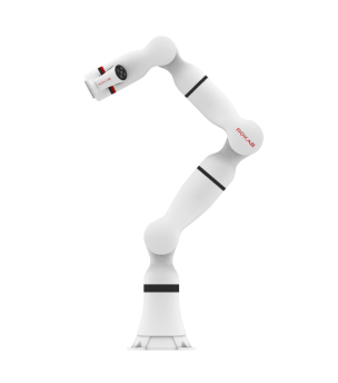
4.3.1.2 Singular position of ER PRO collaborative robot

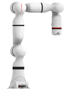
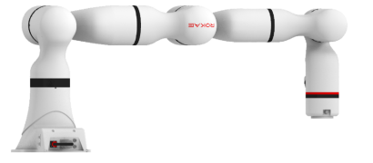
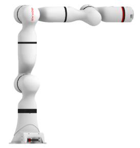
The singularity of ER RPO collaborative robot can be divided into the following cases:

Singularity	Configuration	Explanation
Axis 2 singularity		When the angle of Axis 2 is equal to 0°, the robot is unable to distinguish between the angles of Axis 1 and Axis 3 when solving the inverse kinematics.
Axis 4 singularity		When the angle of Axis 4 is 0°, the robot is restricted to move in the direction parallel to Axis 3 or 5. This singularity causes the robot to lose one degree of freedom at the root of the wrist (the root of the wrist is unable to move along the axis of the arm). In this case, the Axis 3 and Axis 5 positions cannot be obtained through inverse kinematics.
Axis 6 singularity		When the robot’s angle of Axis 6 is equal to 0°, the robot is unable to distinguish between the angles of Axis 5 and Axis 7 when solving the inverse kinematics.
Wrist center singularity		When the wrist center is directly above Axis 1, the robot cannot accurately determine the Axis 1 angle when solving the inverse solution.

Singularity

Configuration

Explanation

Axis 2 singularity

When the angle of Axis 2 is equal to 0°, the robot is unable to distinguish between the angles of Axis 1 and Axis 3 when solving the inverse kinematics.

Axis 4 singularity

When the angle of Axis 4 is 0°, the robot is restricted to move in the direction parallel to Axis 3 or 5. This singularity causes the robot to lose one degree of freedom at the root of the wrist (the root of the wrist is unable to move along the axis of the arm). In this case, the Axis 3 and Axis 5 positions cannot be obtained through inverse kinematics.

Axis 6 singularity

When the robot’s angle of Axis 6 is equal to 0°, the robot is unable to distinguish between the angles of Axis 5 and Axis 7 when solving the inverse kinematics.

Wrist center singularity

When the wrist center is directly above Axis 1, the robot cannot accurately determine the Axis 1 angle when solving the inverse solution.

4.3.2 Singularity avoidance

The singularity problems stem from the robot configuration and cannot be completely avoided. In practical task programming, if the robot must pass through the vicinity of the singularities, it can be considered to reduce some constraints (such as orientation or path accuracy) to make the robot pass through the singularities smoothly.

xCore Control System also provides a variety of singularity avoidance methods:

Method I

Axis 4 Locking

Before enabling the singularity avoidance method, it is necessary to move the robot’s Axis 4 to 0° or ±180°. After this singularity avoidance method is activated, the robot will keep Axis 4 immobile, and perform orientation interpolation in a specialized manner on the premise of ensuring the accurate TCP position. You can refer to the sections of RL command SingAreaLockAxis4 on/off and jog mode.

Method II

Cartesian Sacrifice Orientation Interpolation

After this singularity avoidance method is enabled, the wrist-type singularities can be passed through by changing the morphology of the robot. Note: With this function, the wrist morphology of the robot during motion may differ from that taught during teaching (not only at the teaching points where singularities are traversed, but also potentially at subsequent teaching points).

Method III

Joint Space Interpolation

After this singularity avoidance method is enabled, the control system will perform singularity detection on the subsequent Cartesian trajectories until this function is turned off.

For Cartesian trajectories that do not contain singularities, the robot moves along the ordinary trajectory. When a Cartesian trajectory contains a singularity, the control system detects it and splits the original trajectory P0P1 into three segments: P0Pcut1, Pcut1Pcut2, and Pcut2P1. The segments P0Pcut1 and Pcut2P1 continue to follow the original trajectory and undergo Cartesian interpolation, while the segment Pcut1Pcut2 adopts joint space interpolation to navigate around the singularity. The three trajectory segments are smoothly transitioned using a turning zone, as shown in the following figure.

Singularity avoidance: Schematic diagram of joint space trajectory interpolation

For specific use, you can refer to the RL command SingAreaJointWay.

Note:

Near singularities, the movement amplitude of a robot’s joints tends to be significant. Therefore, you need to confirm whether it is necessary to use a singularity avoidance command. It is preferred to avoid singularities by altering the trajectory points.
When using a singularity avoidance command, it is recommended to first confirm that the robot’s trajectory with the singularity avoidance command enabled satisfies the operational requirements before performing the official operation.
Near singularities, the movement amplitude of a robot’s joints tends to be significant, so you need to confirm the surrounding environment before using it.
In view of the above reasons, if the robot operating point or program run logic is affected by external signals, it is recommended to carefully confirm the program logic and trajectory before use.

The specific characteristics of the above three singularity avoidance methods are as follows:

Mode and Feature	Axis 4 Locking	Cartesian Sacrifice Orientation Interpolation	Joint Space Interpolation
Motion feature	1. Before enabling this command, it is necessary to move the robot’s Axis 4 to 0° or ±180°. 2. After this command is enabled, the robot keeps Axis 4 immobile for subsequent motion commands.	1. After enabling this command, the robot will change the wrist morphology, resulting in a change in the tool orientation to allow passage through trajectories with wrist singularities. 2. The wrist morphology during motion may sometimes differ from the taught morphology, not only at the teaching points where singularities are traversed, but also potentially at subsequent teaching points.	1. The sections of the trajectory before and after the singularity adopt joint interpolation (MoveAbsJ) for movement, while the remaining sections retain the original Cartesian trajectory’s movement method. A turning zone is used for a smooth transition between the above two movement methods.
Trajectory form change	1. Position trajectory remains unchanged. 2. Special orientation interpolation methods are employed.	1. Position trajectory remains unchanged. 2. Orientation interpolation method is altered.	1. Position trajectory is altered. 2. Orientation trajectory is altered.
Reachability of target points	The robot’s workspace is partially reachable. Specifically, partial target points are reachable when the Axis 4 is set at 0° or ±180°.	The robot’s workspace is partially reachable.	The robot’s entire workspace is reachable.
Turning zone feature	1. Generating turning zones between similar trajectories is supported, specifically, between the motion trajectories when SingAreaLockAxis4 is on and off. 2. Generating turning zones between different types of trajectories is not supported, that is, generating turning zones is not supported between motion trajectories that precede or follow the activation of the SingAreaLockAxis4 on/off command.	1. Generating turning zones between similar trajectories is supported, specifically, between the motion trajectories when SingAreaWrist is on and SingAreaWrist4 is off. 2. For different types of trajectories, generating turning zones is supported between joint space trajectories and singularity avoidance trajectories, while generating turning zones is not supported between Cartesian space trajectories and singularity avoidance trajectories.	Generating turning zones is supported between singularity avoidance trajectories, as well as between singularity avoidance trajectories and ordinary trajectories.
Lookahead feature	The lookahead mechanism is interrupted. Specifically, the SingAreaLockAxis4 on/off serves as a blocking command, and the control system will only continue to parse singularity avoidance commands after the robot has completed the trajectory preceding the activation of the SingAreaLockAxis4 on command. Similarly, the control system will resume parsing subsequent commands only after the robot has executed the motion command preceding the activation of the SingAreaLockAxis4 off command.	The lookahead mechanism is not interrupted.	The lookahead mechanism is not interrupted.
Whether the singularity avoidance is mandatory	Mandatory. After the axis locking, all Cartesian motion commands are interpolated by the special interpolation form corresponding to the locked axis until the axis locking function is turned off.	Mandatory. After the sacrifice orientation singularity avoidance is enabled, all Cartesian motion commands are interpolated by the special interpolation form corresponding to the locked axis until the sacrifice orientation singularity avoidance function is turned off.	Not mandatory. After this singularity avoidance is enabled, the control system automatically detects whether there are singularities in each Cartesian motion trajectory. The trajectory that only contains singularities will adopt special forms of interpolation, while the trajectory that does not contain singularities still employs the motion form of ordinary trajectories for interpolation. Note: The calculation amount of the control system will increase after this function is enabled, so this function is not enabled generally unless necessary.
Applicable scenarios	1. The trajectory where the flange remains parallel to the base or moves along the z-axis of the base. 2. During the robot’s movement, it is permissible to keep Axis 4 immobile, such as stacking.	Do not mind the orientation accuracy of trajectories, nor how the robot reaches the target points, only pursuing the ability to reach the Cartesian position of the target points.	Do not mind the position accuracy and orientation accuracy of trajectories, nor how the robot reaches the target points, only pursuing the ability to reach the target points.
Supported model	Industrial standard six-axis series (XB, NB model), collaborative xMate CR/SR	Industrial standard six-axis series (XB, NB model), collaborative xMate CR/SR	Industrial standard six-axis series (XB, NB model)
Whether Jog is supported	Supported	Not supported	Not supported

Mode and Feature

Axis 4 Locking

Cartesian Sacrifice Orientation Interpolation

Joint Space Interpolation

Motion feature

1. Before enabling this command, it is necessary to move the robot’s Axis 4 to 0° or ±180°.

2. After this command is enabled, the robot keeps Axis 4 immobile for subsequent motion commands.

1. After enabling this command, the robot will change the wrist morphology, resulting in a change in the tool orientation to allow passage through trajectories with wrist singularities.

2. The wrist morphology during motion may sometimes differ from the taught morphology, not only at the teaching points where singularities are traversed, but also potentially at subsequent teaching points.

1. The sections of the trajectory before and after the singularity adopt joint interpolation (MoveAbsJ) for movement, while the remaining sections retain the original Cartesian trajectory’s movement method. A turning zone is used for a smooth transition between the above two movement methods.

Trajectory form change

1. Position trajectory remains unchanged.

2. Special orientation interpolation methods are employed.

1. Position trajectory remains unchanged.

2. Orientation interpolation method is altered.

1. Position trajectory is altered.

2. Orientation trajectory is altered.

Reachability of target points

The robot’s workspace is partially reachable. Specifically, partial target points are reachable when the Axis 4 is set at 0° or ±180°.

The robot’s workspace is partially reachable.

The robot’s entire workspace is reachable.

Turning zone feature

1. Generating turning zones between similar trajectories is supported, specifically, between the motion trajectories when SingAreaLockAxis4 is on and off.

2. Generating turning zones between different types of trajectories is not supported, that is, generating turning zones is not supported between motion trajectories that precede or follow the activation of the SingAreaLockAxis4 on/off command.

1. Generating turning zones between similar trajectories is supported, specifically, between the motion trajectories when SingAreaWrist is on and SingAreaWrist4 is off.

2. For different types of trajectories, generating turning zones is supported between joint space trajectories and singularity avoidance trajectories, while generating turning zones is not supported between Cartesian space trajectories and singularity avoidance trajectories.

Generating turning zones is supported between singularity avoidance trajectories, as well as between singularity avoidance trajectories and ordinary trajectories.

Lookahead feature

The lookahead mechanism is interrupted. Specifically, the SingAreaLockAxis4 on/off serves as a blocking command, and the control system will only continue to parse singularity avoidance commands after the robot has completed the trajectory preceding the activation of the SingAreaLockAxis4 on command. Similarly, the control system will resume parsing subsequent commands only after the robot has executed the motion command preceding the activation of the SingAreaLockAxis4 off command.

The lookahead mechanism is not interrupted.

Whether the singularity avoidance is mandatory

Mandatory. After the axis locking, all Cartesian motion commands are interpolated by the special interpolation form corresponding to the locked axis until the axis locking function is turned off.

Mandatory. After the sacrifice orientation singularity avoidance is enabled, all Cartesian motion commands are interpolated by the special interpolation form corresponding to the locked axis until the sacrifice orientation singularity avoidance function is turned off.

Not mandatory. After this singularity avoidance is enabled, the control system automatically detects whether there are singularities in each Cartesian motion trajectory. The trajectory that only contains singularities will adopt special forms of interpolation, while the trajectory that does not contain singularities still employs the motion form of ordinary trajectories for interpolation.

Note: The calculation amount of the control system will increase after this function is enabled, so this function is not enabled generally unless necessary.

Applicable scenarios

1. The trajectory where the flange remains parallel to the base or moves along the z-axis of the base.

2. During the robot’s movement, it is permissible to keep Axis 4 immobile, such as stacking.

Do not mind the orientation accuracy of trajectories, nor how the robot reaches the target points, only pursuing the ability to reach the Cartesian position of the target points.

Do not mind the position accuracy and orientation accuracy of trajectories, nor how the robot reaches the target points, only pursuing the ability to reach the target points.

Supported model

Industrial standard six-axis series (XB, NB model), collaborative xMate CR/SR

Industrial standard six-axis series (XB, NB model)

Whether Jog is supported

Supported

Not supported

4.4 Turning zone

The motion of a robot typically involves sequentially executing multiple trajectories programmed and set by the user. Usually, these trajectories are not smoothly connected, and there are various "spikes" between them. The presence of these "spikes" forces the robot to first stop at the end of a trajectory before starting the next trajectory. To enable continuous motion between trajectories, it is necessary to eliminate such "spikes", and different trajectories can be smoothly connected by generating turning zones. See the following figure:

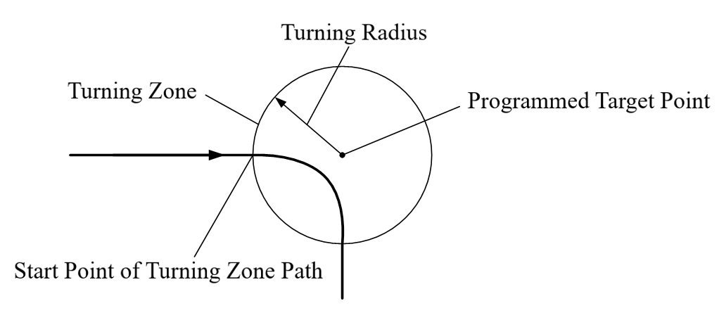
The turning zone type includes Cartesian space turning zone and joint space turning zone. For the detailed definition and specific parameters of the turning zone, please refer to the section below, "RL Command"-"zone".

4.5 Lookahead mechanism

Lookahead means that the control system handles the subsequent program commands in advance when the robot is executing the current command during robot movement.

The introduction of the lookahead mechanism can be advantageous in the following aspects:

Obtain the speed of the front trajectory, the acceleration requirements, and the constraints of the robot itself, so as to plan the control strategy for optimal performance;
Plan the turning trajectory of the turning zone according to the settings of the programmed turning zone;
Acquire an abnormal state near the soft limit/boundary and singular points, etc., so that it can be handled in advance;

For a more detailed introduction to the lookahead mechanism, refer to the section below, "Programming"-"About RL program"-" RL program debugging".

4.6 Force control

4.6.1 Introduction to force control

The robot force control is a process of interaction between the robot end-effector and forces in the external environment. During non-contact robot motion control, only the position control process (velocity and accuracy) is considered. When there is contact with the environment, pure position control requires very high accuracy of the robot and the environment to avoid damage to the robot and the environment caused by contact forces resulting from positional deviations.

Unlike pure position control, robot force control introduces a force/torque feedback loop when interacting with the environment. The loop is used to change the motion characteristics of the robot, which enables dynamic interaction with the external environment. When there is deviation or uncertainty between the robot and the external environment, the force control will intelligently adjust the preset position trajectory to eliminate the internal force caused by the position deviation and ensure a smooth and safe interaction process

4.6.2 Impedance control

Compared with traditional industrial robots, xMate collaborative robot is equipped with torque sensors in its joints, which enable it to sense joint torque precisely. The joint torque information allows the xMate collaborative robot to achieve force control through impedance, making the robot have compliant interactive behaviors. This means the interaction between the robot and the environment is like a virtual spring stiffness and damping system. At this point, the robot is sensitive to external forces, which can cause the robot to deviate from a predetermined trajectory. When the external forces disappear, the robot can rebound to some extent.

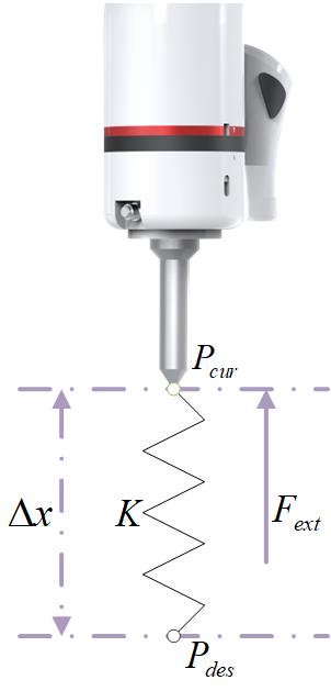
In the process of impedance motion, the actual position of the robot will deviate from the desired position when affected by the external forces in the environment. The deviation depends on the impedance stiffness and the external forces, and it can be calculated through the ratio between the external force and the impedance stiffness. As shown above, in the impedance control mode, with impedance stiffness set to K and under the action of external force Fext, the robot’s current position Pcur will deviate from the desired position Pdes, and the position deviation is Δx. The impedance force caused by this deviation and the external force will eventually reach an equilibrium.

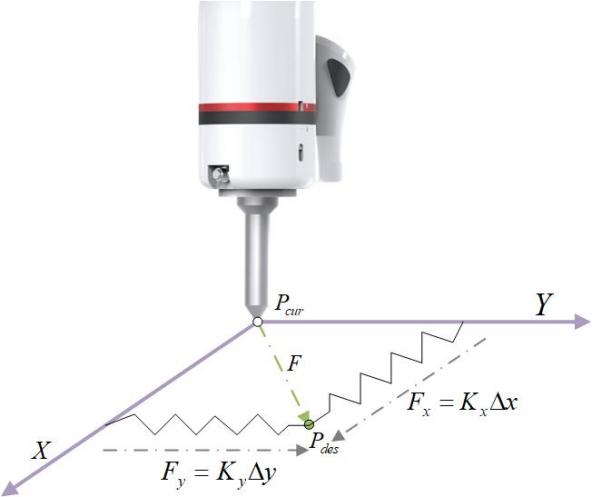
The impedance stiffness in each direction can be set individually, and the impedance force in each direction is the product of the impedance stiffness and the position deviation in this direction. The impedance forces in all directions are ultimately combined to form the total impedance force. In the figure below, the robot’s current position Pcur deviates from the desired position Pdes due to the action of external forces in the impedance mode. In the X and Y directions, the deviations are Δx and Δy, the impedance stiffnesses are Kx and Ky, and the impedance forces are Fx and Fy, respectively. The total impedance force F = Fx + Fy.

4.6.3 Force control search

When assembling work objects, humans can feel the change in force by hand. If an obstruction (a work object is stuck) is detected, humans will try shaking to ensure a smooth installation. Force control allows the robot to do the same thing, i.e. overlay. The robot supports sine overlay rotating around an axis and Lissajous overlay within a plane. Overlay is an additional movement superimposed on the robot’s predetermined motion. Overlay allows the robot to exhibit a certain degree of shake, enabling it to better overcome obstacles during assembly.

Below is a sine overlay:

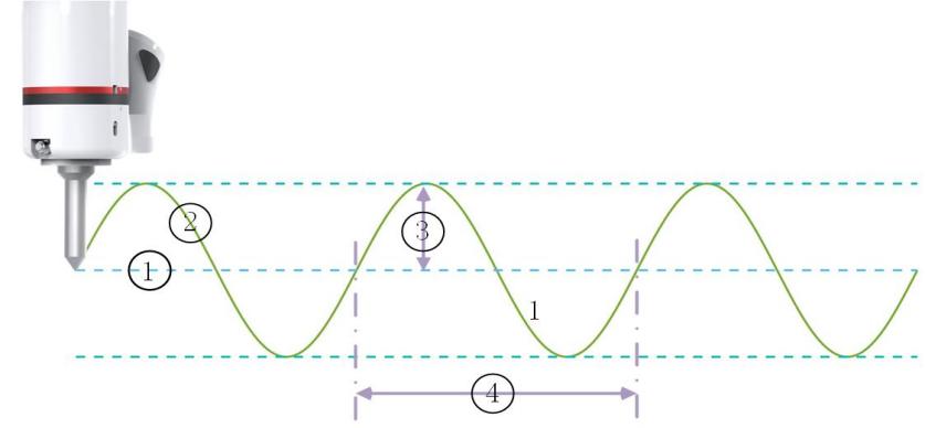
1	Desired trajectory	2	Actual trajectory (desired trajectory + overlay)
3	Overlay amplitude	4	Overlay period

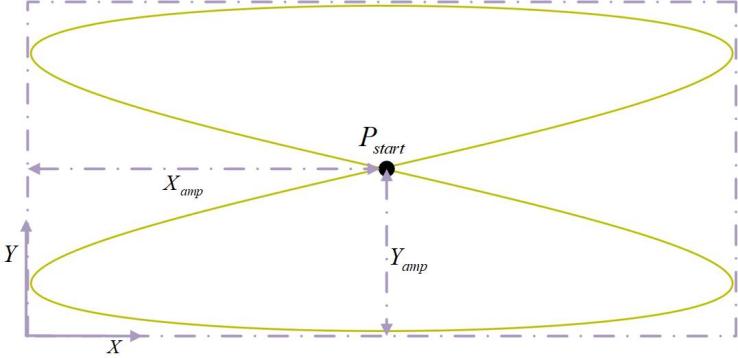
Lissajous overlay refers to the application of sine search motions in two perpendicular directions within a plane, and the frequencies of the two overlays are often proportional. For example, below shows the Lissajous overlay in the XY plane, where the frequency ratio of x- and y-direction overlay are 2:1. The center point Pstart is the desired pose, Xamp is the amplitude of the x-direction overlay, and Yamp is the amplitude of the y-direction overlay.

4.6.4 Force control application

The application scenarios of force control for industrial robots can roughly be divided into two categories: constant force tracking and force-controlled assembly.

4.6.4.1 Constant force tracking

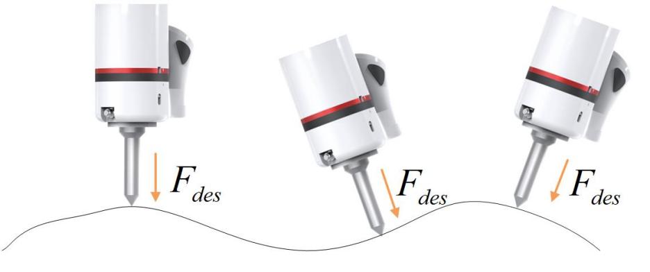
Below is a constant force tracking scenario. The robot ensures a constant contact force Fdes with the surface, while the robot can conform to the surface curve. Main applications of constant force tracking include grinding and deburring.

4.6.4.2 Force-controlled assembly

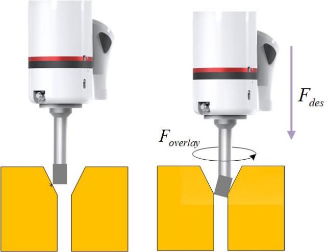
If pure position control is used during the assembly, the robot may easily collide with the work object due to position and modeling errors, which can cause damage to the work object or the robot. But with force control, the robot will try to overlay (shake) to overcome the obstruction when it senses an external force over the limit (work object jamming), thus allowing smooth work object installation. As shown below, the position control on the left results in a collision during assembly, while the force control on the right pushes the robot into the assembly hole through the desired force Fdes, and the jamming is prevented through overlay Foverlay.